Optimize training performance with Reduction Server on Vertex AI

As deep learning models become more complex and the size of training datasets keeps increasing, training time has become one of the key bottlenecks in the development and deployment of ML systems. Even if you have access to a GPU, with a large dataset it can take days or weeks for a deep learning model to converge. Using the right hardware configuration can reduce training time to hours, or even minutes. And a shorter training time makes for faster iteration to reach your modeling goals.

To speed up training of large models, many engineering teams are adopting distributed training using scale-out clusters of ML accelerators. However, distributed training at scale brings its own set of challenges. Specifically, limited network bandwidth between nodes makes optimizing performance of distributed training inherently difficult, particularly for large cluster configurations.

In this article, we introduce Reduction Server, a new Vertex AI feature that optimizes bandwidth and latency of multi-node distributed training on NVIDIA GPUs for synchronous data parallel algorithms. Synchronous data parallelism is the foundation of many widely adopted distributed training frameworks, including TensorFlow’s MultiWorkerMirroredStrategy, Horovod, and PyTorch Distributed. By optimizing bandwidth usage and latency of the all-reduce collective operation used by these frameworks, Reduction Server can decrease both the time and cost of large training jobs.

This article covers key terminology in the field of distributed training, such as data parallelism, synchronous training, and all-reduce, and shows how to configure and submit Vertex Training jobs that utilize Reduction Server. Additionally, we provide sample code for using Reduction Server to tune a BERT model on the MNLI dataset.

Overview of distributed data parallel training on GPUs

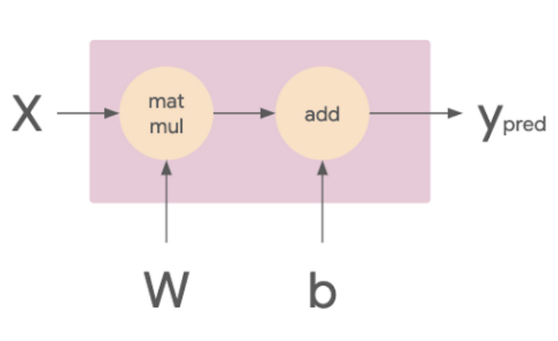
Imagine you have a simple linear model, which you can think of in terms of its computational graph. In the image below, the matmul op takes in the X and W tensors, which are the training batch and weights respectively. The resulting tensor is then passed to the add op with the tensor b, which is the model’s bias terms. The result of this op is Ypred, which is the model’s predictions.

We want a way of executing this computational graph such that we can leverage multiple workers. One option would be putting different layers of your model on different machines or devices, which is a type of model parallelism. Alternatively, you could distribute your dataset such that each worker processes a different portion of the input batch on each training step with the same model, which is known as data parallelism. Or you might do a combination of both. Generally, model parallelism works best for models where there are independent parts of computation that can run in parallel. Data parallelism works with any model architecture, which makes it more widely adopted for distributed training.

The following image shows an example of data parallelism. The input batch X is split in half, and one slice is sent to GPU 0 and the other to GPU 1. In this case, each GPU calculates the same ops but on different slices of the data.

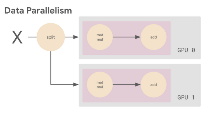
The subsequent gradient updates will happen in a synchronous manner:

• Each worker device performs the forward pass on a different slice of the input data to compute the loss.
• Each worker device computes the gradients based on the loss function.
• These gradients are aggregated (reduced) across all of the devices.
• The optimizer updates the weights using the reduced gradients, thereby keeping the devices in sync.

You can use data parallelism to speed up training for a single machine with multiple GPUs, or for multiple machines, each with potentially multiple GPUs. For the rest of this discussion we assume that compute workers map to GPU devices one-to-one. For example, a single compute node with two GPU devices has two workers. And a four node cluster where each node has two GPU devices manages eight workers.

A key aspect of data parallel distributed training is the gradient aggregation. Because each worker cannot proceed to the next training step until all the other workers have finished the current step, this gradient calculation becomes the main overhead in distributed training for synchronous strategies. To perform this gradient aggregation, most widely adopted distributed training frameworks leverage a synchronous all-reduce collective communication operation.

All-reduce is a collective communication operation that reduces a set of arrays on distributed workers to a single array that is then re-distributed back to each worker. In gradient aggregation the reduction operation is a summation.

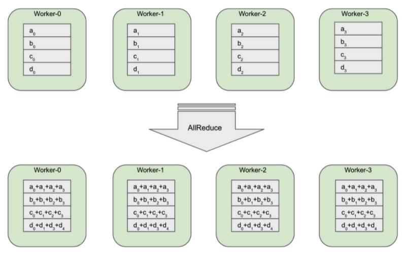
The diagram above shows 4 GPU workers. Before the all-reduce operation, each worker has an array of gradients that were calculated on its batch of training data. Because each worker received a different batch of training data, the subsequent gradient arrays (g₀, g₁, g₂, g₃) are all different.

After the all-reduce operation is completed, each worker will have the same array. This array is computed by aggregating (a summation) gradient arrays across all workers.

There are many different algorithms for efficiently implementing this aggregation. In general, workers communicate and exchange gradients with each other over a topology of communication links. The choice of the topology and the gradient exchange pattern impacts the bandwidth required by the algorithm and its latency.

One simple example of an all-reduce implementation is called Ring All-reduce, where the workers form a logical ring and communicate only with their immediate neighbors.

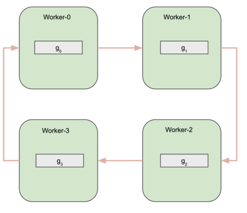
The algorithm can be logically divided into two phases:

1. Reduce-scatter phase
2. All-gather phase

At the start of the Reduce-scatter phase the gradient array on each worker is divided into N equal size blocks, where N is the number of workers, which in this case is 4.

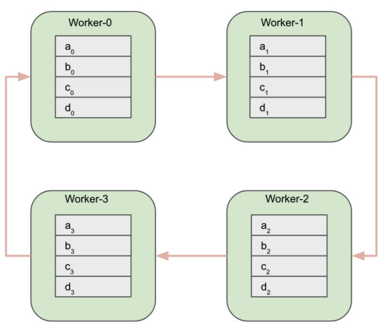
In the next step, each worker simultaneously sends one of these blocks to one neighbor and receives a different block from the other neighbor.

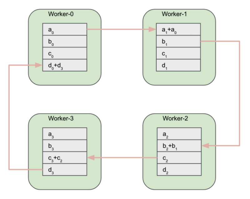
Worker-0 sends the a₀ block to Worker-1. Worker-1 sends the b₁ block to Worker-2. Worker-2 sends the c₂ block to Worker-3. And finally, Worker-3 sends the d₃ block to Worker-0. As noted earlier, all send and receive operations in the ring are simultaneous.

When this step completes, each worker can perform a partial reduction using the block received from its neighbor.

After the partial reduction, workers exchange partially reduced blocks. Worker-1 sends the reduced a₁+a₀ block to Worker-2. Worker-2 sends the reduced b₂+b₁ block to Worker-3. And so on.

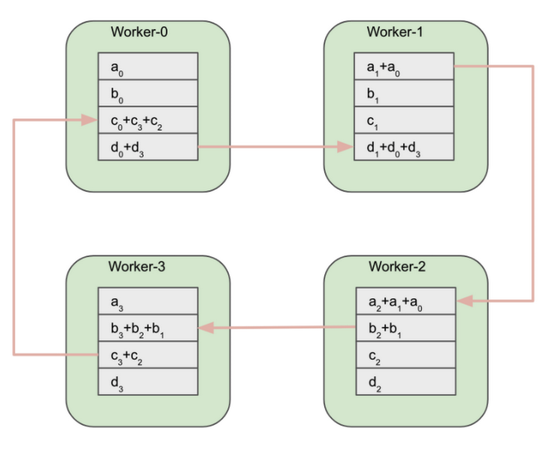
At the end of the Reduce-scatter phase, each worker will have one fully reduced block of the original arrays.

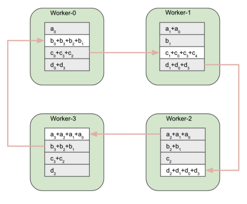
At this point, the All-gather phase of the algorithm starts.

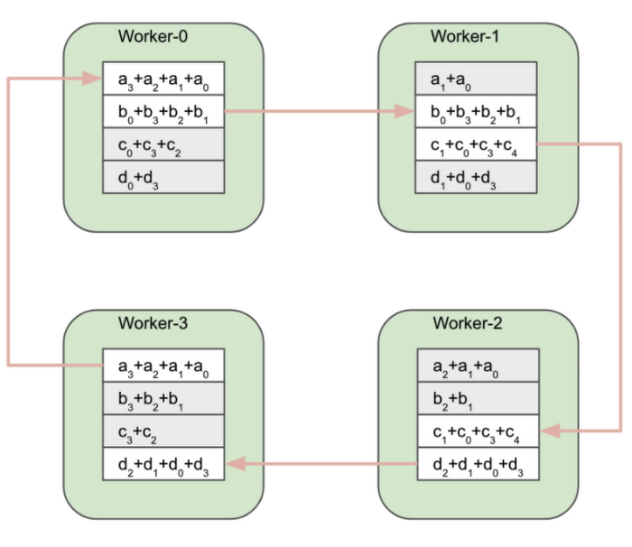
Worker-0 sends the fully reduced b₀+b₃+b₂+b₁ block to Worker-1. Worker-1 sends the c₁+c₀+c₃+c₄ block to Worker-2 and so on.

At the end of the All-gather phase all workers have the same fully reduced array.

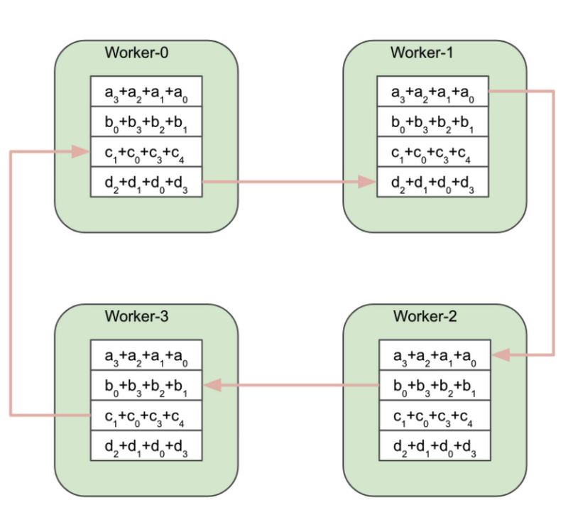
During the Reduce-scatter phase, each worker sends and receives N-1 blocks of data, where N is the number of workers. The same number of blocks are exchanged during the All-gather phase. In total, 2(N-1) blocks of data are sent and received by each worker during the Ring All-reduce algorithm. If the size of the gradient array is K bytes then the number of bytes sent and received during the all-reduce operation is (2(N-1)/N)*K.

The downside of the Ring All-reduce is that the latency of the algorithm scales linearly with the number of workers, effectively preventing scaling to larger clusters. Other implementations of all-reduce based on tree topologies can achieve logarithmic scaling.

The Reduction Server algorithm

The Vertex Reduction Server uses a distinctive communication link topology by introducing an additional worker role, a reducer. Reducers are dedicated to one function only: aggregating gradients from workers. Reducers don’t calculate gradients or maintain model parameters. Because of their limited functionality, reducers don’t require a lot of computational power and can run on relatively inexpensive compute nodes.

The following diagram shows a cluster with four GPU workers and five reducers. GPU workers maintain model replicas, calculate gradients, and update parameters. Reducers receive blocks of gradients from the GPU workers, reduce the blocks and redistribute the reduced blocks back to the GPU workers.

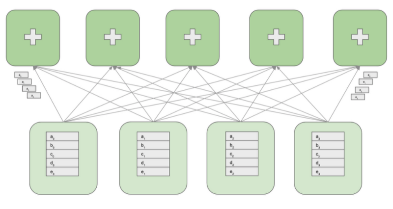
To perform the all-reduce operation, the gradient array on each GPU worker is first partitioned into M blocks, where M is the number of reducers. A given reducer processes the same partition of the gradient from all GPU workers. For example, as shown on the above diagram, the first reducer reduces the blocks a₀ through a₃ and the second reducer reduces the blocks b₀ through b₃. After reducing the received blocks, a reducer sends back the reduced partition to all GPU workers.

Assuming that the size of a gradient array is K bytes, each node in the topology sends and receives K bytes of data. That is almost half the data that the Ring and Tree based all-reduce implementations exchange. An additional advantage of Reduction Server is that its latency does not depend on the number of workers.

The below table compares data transfer and latency characteristics of Reduction Server compared to Ring and Tree based all-reduce algorithms. Recall that N is the number of workers, and K is the size of the gradient array (bytes).

Using Reduction Server with Vertex Training

Reduction Server can be used with any distributed training framework that uses the NVIDIA NCCL library for the all-reduce collective operation. You do not need to change or recompile your training application.

To use Reduction Server with Vertex Training custom jobs you need to:

• Choose a topology of Vertex Training worker pools.
• Install the Reduction Server NVIDIA NCCL transport plugging in your training container image.
• Configure and submit a Vertex Training custom job that includes a Reduction Server worker pool.

Each of these steps is discussed in detail in the following sections.

Choosing a topology of Vertex Training worker pools

To run a multi-worker training job with Vertex AI, you specify multiple machines (nodes) in a training cluster. The training service allocates the resources for the machine types you specify. Your running job on a given node is called a replica. A group of replicas with the same configuration is called a worker pool. Vertex AI provides up to 4 worker pools to cover the different types of machine tasks. When using Reduction Server the first three worker pools are used.

Worker pool 0 configures the Primary, chief, scheduler, or “master”. This worker generally takes on some extra work such as saving checkpoints and writing summary files. There is only ever one chief worker in a cluster, so your worker count for worker pool 0 will always be 1.

Worker pool 1 is where you configure the rest of the workers for your cluster.

Worker pool 2 manages Reduction Server reducers. When choosing the number and type of reducers, you should consider the network bandwidth supported by a reducer replica’s machine type. In GCP, a VM’s machine type defines its maximum possible egress bandwidth. For example, the egress bandwidth of the n1-highcpu-16 machine type is limited at 32 Gbps.

Because reducers perform a very limited function, aggregating blocks of gradients, they can run on relatively low-powered and cost effective machines. Even with a large number of gradients this computation does not require accelerated hardware or high CPU or memory resources. However, to avoid network bottlenecks, the total aggregate bandwidth of all replicas in the reducer worker pool must be greater or equal to the total aggregate bandwidth of all replicas in worker pools 0 and 1, which host the GPU workers.

For example, if you run your distributed training job on eight GPU equipped replicas that have an aggregate maximum bandwidth of 800 Gbps (GPU equipped VMs can support up to 100 Gbps egress bandwidth) and you use a reducer with 32 Gbps egress bandwidth, you will need at least 25 reducers.

To maintain the size of the reducer worker pool at a reasonable level it’s recommended that you use machine types with 32 Gbps egress bandwidth, which is the highest bandwidth available to CPU only machines in Vertex Training. Based on the testing performed on a number of mainstream Deep Learning models in Computer Vision and NLP domains, we recommend using the reducers with 16-32 vCPUs and 16-32 GBs of RAM. A good starting configuration that should be optimal for a large spectrum of distributed training scenarios is the n1-highcpu-16 machine type.

Installing the Reduction Server NVIDIA NCCL transport plugin

Reduction Server is implemented as an NVIDIA NCCL transport plugin. This plugin must be installed on the container image that is used to run your training application.

The code accompanying this article includes a sample Dockerfile that uses the Vertex pre-built TensorFlow 2.5 GPU Docker image as a base image, which comes with the plugin pre-installed.

You can also install the plugin directly by including the following in your Dockerfile:

Configuring Vertex Training jobs using Reduction Server

First, import and initialize the Vertex SDK.

Next, you’ll specify the configuration for your custom job. In the following spec, there are three worker pools defined:

• Worker pool 0 has one worker with 4 NVIDIA A100 Tensor Core GPUs.
• Worker pool 1 defines an additional 7 GPU workers, resulting in 8 GPU workers overall.
• Worker pool 2 specifies 14 reducers of machine type n1-highcpu-16.

Note that worker pools 0 and 1 run your training application in a container image configured with the Reduction Server NCCL transport plugin. Worker pool 2 uses the Reduction Server container image provided by Vertex AI.

Next, create and run a CustomJob.

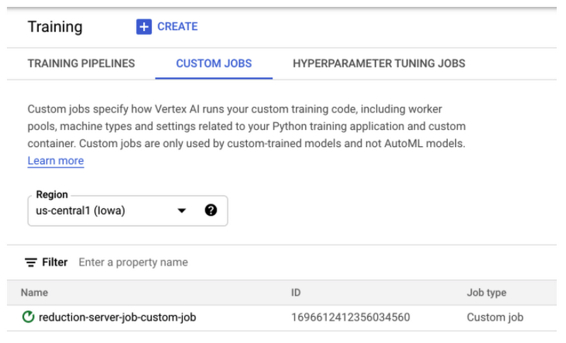
In the Training section of your cloud console under the CUSTOM JOBS tab you’ll see your training job:

Analyzing performance and cost benefits of Reduction Server

The impact Reduction Server has on the elapsed time of your training job and the potential resulting cost savings depend on the characteristics of your training workload.

In general, computationally intensive workloads that require a large number of GPUs to complete training in a reasonable amount of time, and where the trained model has a large number of parameters, will benefit the most. This is because the latency for standard ring and tree based all-reduce collectives is proportional to both the number of GPU workers and the size of the gradient array. Reduction Server optimizes both: latency does not depend on the number of GPU workers, and the quantity of data transferred during the all-reduce operation is lower than ring and tree based implementations.

One example of a workload that fits this category is pre-training or fine-tuning large language models like BERT. Based on exploratory experiments, you can expect a 30%-40% reduction in training time for this type of workload.

The diagram below shows the results of fine tuning a BERT model from the TensorFlow Model Garden on the MNLI dataset using eight GPU worker nodes each equipped with 8 NVIDIA A100 Tensor Core GPUs.

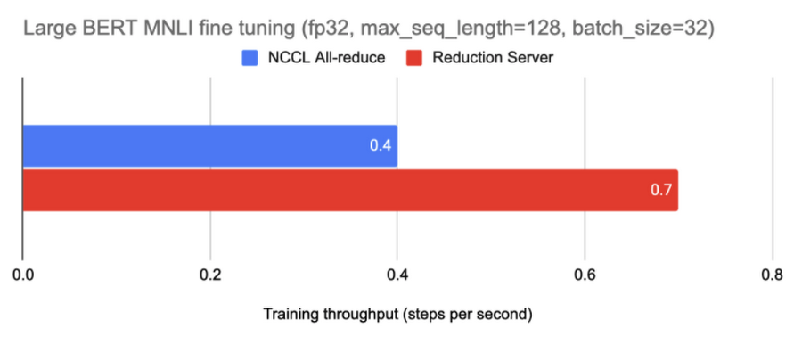
In this experiment, adding 20 reducer nodes increased the training throughput from around 0.4 steps per second to 0.7 steps per second.

A reduction in training time can also translate into a reduction in training costs. However, in many mission critical scenarios the shortened training cycle carries a much higher business value than raw savings in the usage of compute resources. For example, it allows you to train a model with higher predictive performance within the constraints of a deployment window.

The table below reports the per step training costs for the above experiment. These cost estimates are based on Vertex AI pricing for custom-trained models in the Americas region.

What’s next

In this article you learned how the Vertex Reduction Server architecture provides a novel all-reduce implementation that minimizes latency and data transferred by utilizing a specialized worker type that is dedicated to gradient aggregation. If you’d like to try out a working example from start to finish, you can take a look at this notebook. It’s time to use Reduction Server and run some experiments of your own. Happy distributed training!