Creating a serverless pipeline for real-time market data

Editor’s note: This is the second part in our special series on working with market data in Google Cloud. This post highlights how we leveraged serverless components to build a flexible data ingestion pipeline. Check out the first post on visualizing real-time market data in the cloud.

Capital markets firms must rapidly extract insights from unbounded real-time datasets. A firm’s market data pipelines should weigh the end user’s data access requirements as a central design consideration, but oftentimes the rigidity of delivery mechanisms and analytical tools block this goal. Serverless data offerings can solve this problem by removing operational friction when introducing a new, well-suited tool. This makes it simple for one data pipeline to serve separate user goals–say, one for training a real-time machine learning model and another for analyzing historical data.

With a serverless data pipeline, capital markets firms can focus on insights, not infrastructure, and stay ahead in a fast-moving industry. In this post, you’ll see best practices for real-time data ingestion using CME Group’s Smart Stream top-of-book (ToB) JSON feed. The reference architecture considers data usage patterns and schema when selecting storage and transport options. It also encapsulates business logic in Cloud Functions to increase the speed of development and to offload operational complexities. These patterns and designs can be applied to a wide variety of use cases.

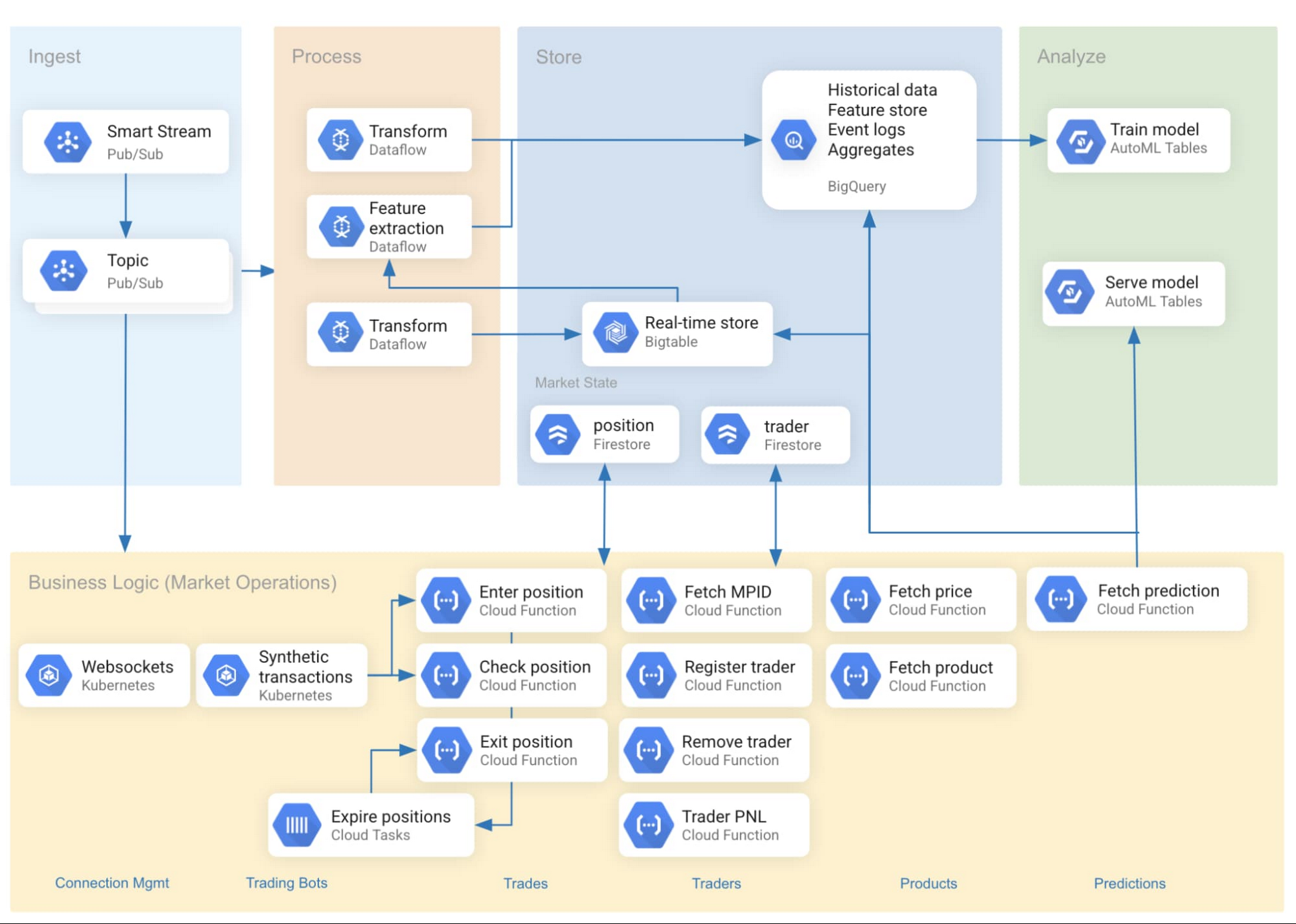
Figure 1 depicts the ingestion pipeline’s reference architecture.

Figure 1: Reference architecture

How we set up real-time data ingestion

The source of the real-time data we used is Smart Stream, a service available on Google Cloud from CME Group. The data originates with the CME Globex trading platform as a multicast stream running over UDP. The instrument price data is forwarded over an interconnect to different Pub/Sub topics, each corresponding to a single product, like silver or orange juice concentrate futures.

Pub/Sub is serverless and tightly integrated with other Google Cloud services. It’s also fully managed by Google, alleviating users from many scaling, planning, and reliability concerns. Google provides open-source Dataflow templates to ingest data from Pub/Sub to various sinks such as BigQuery and Cloud Storage.

Bigtable was leveraged as a real-time data store, serving most recent data and features to a prediction endpoint. (The endpoint passes this data to machine learning models hosted on Google Cloud’s AI Platform). In parallel, we use BigQuery as a scalable analytics warehouse. Pub/Sub data was streamed to both sinks with separate Dataflow jobs.

Figure 2 is a shell snippet launches a Dataflow job with a Google-provided template for PubSub-to-BigQuery pipelines:

Figure 2: Launching a Dataflow template to ingest messages from Pub/Sub to BigQuery

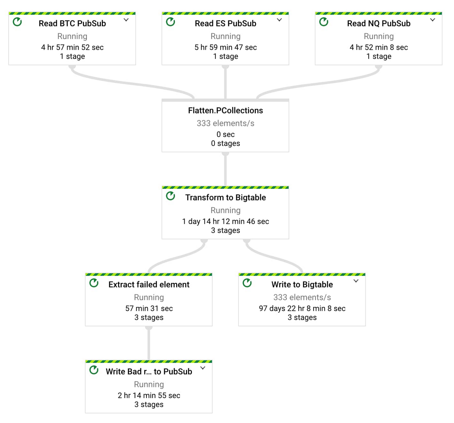
Figure 3 depicts a Dataflow pipeline with three input Pub/Sub topics (one per trading instrument) and Bigtable as a sink:

Figure 3: Dataflow job graph

The class in Figure 4 defines an Apache Beam pipeline to ingest data from a single topic (i.e., product code) and write to Bigtable:

Figure 4: Apache Beam ingestion pipeline to Bigtable

At first glance, the app’s predictive models and web front-end charts are similar in their demand for data freshness. On further inspection, however, a difference emerges–the charts can use the Smart Stream price data directly without an intervening data store. So for front-end delivery, we settled on Pub/Sub via websockets.

Using Pub/Sub with serverless ingestion components offered architectural flexibility and removed operational complexity as a constraint. Data coming from one Pub/Sub topic can be stored in Bigtable for machine learning or in BigQuery for analytics, in addition to being sent directly over websockets to power rapidly changing visualizations.

Storage and schema considerations

Ideally, the time spent managing data is minimal compared to the time spent using data. If schema design and storage architecture is executed properly, users will feel that the data is working for them, rather than them working for the data.

Row key design is critical to any Bigtable pipeline. Our key concatenates a product symbol with a reverse timestamp, which is optimized for our access pattern (“fetch N most recent records”) while avoiding hotspotting.

In order to reverse the timestamp, we subtract it from the programming language’s maximum value for long integers (such as Java’s java.lang.Long.MAX_VALUE). This forms the key: <SYMBOL>#<INVERTED_TIMESTAMP>. A product code’s most recent events appear at the start of the table, speeding up the query response time. This approach accommodates our primary access pattern (which queries multiple recent product symbols)–but may yield poor performance for others. A post on Bigtable schema design for time series data has additional concepts, patterns and examples.

Figure 5 shows a sample data point ingested into Bigtable:

Figure 5: Representation of a market data record within Bigtable

While Bigtable is well-suited to deliver low-latency data to machine learning models, we also needed a more analytically tuned query engine for longer-lookback insights. BigQuery was a natural fit because of its serverless and scalable nature, as well as its integration with tools such as AutoML.

When designing, we considered three options for preparing the BigQuery data for visualization as classic OHLC “candlesticks.” First, we could store the nested Pub/Sub JSON into BigQuery and write a complex SQL query to unnest and aggregate. Second, we could write a view that unnests, and then write a simpler SQL query that aggregates (without unnesting). Third, we could develop and run a Dataflow job to unnest Pub/Sub records into a “flat” format for storage in BigQuery, and could then aggregate with a simple SQL query.

Though the third option may represent a superior design longer term, time constraints steered us towards the second option. The BigQuery view was simple to set up, and the team got productive quickly when querying against the flattened schema. Thanks to a DATE partition filter, the SQL view definition scans only the most recent day from the underlying table storing the quotes. This dramatically improves performance of the queries against the view.

A sample of the data transformation and views for this specific chart using the second methodology are shown in Figures 6 and 7.

Figure 6: SQL view definition to flatten original source records

Figure 7: SQL view definition that generates OHLC bars (“candlesticks”)

Because both Bigtable and BigQuery are serverless, the maintenance of each storage solution is minimal, and more time can be spent deriving and delivering value from the data, rather than capacity planning around procurement of storage arrays and operational complexities.

Market data microservices

Cloud Functions offer developers two primary benefits. First, they provide the ability to bypass non-differentiating low-level implementation details in favor of business-specific code. Second, they support flexible use of data by encapsulating business logic outside of the database. In our pipeline, we accordingly used Cloud Functions for isolated, task-specific code chunks.

One example is our pipeline’s Fetch Prediction function, which retrieves trade records from Bigtable and extracts first-order features (mean, sum, max, etc) for input to the machine learning model. This enables rapid predictions that are used by the bots to make algorithmic trading decisions in near real-time.

This is demonstrated in Figure 8.

Figure 8: Python routine to fetch predictions at runtime

Fetch Candles is a Cloud Function that fetches a recent price summary from BigQuery detailing the opening, closing, highest and lowest price observed for each minute. To improve the request-response performance, we enabled HTTP(s) load balancing with a serverless network endpoint group for our app, and then optimized delivery with Cloud CDN. Configured this way, Fetch Candles will query BigQuery only for the first request for a given minute and product code. Subsequent requests will be delivered from the Cloud CDN cache, until the maximum cache TTL of one minute is reached. This can significantly reduce the overall volume of query executions as web client traffic scales up. Since the data is in a lookback window, there’s no functional necessity for BigQuery to calculate the aggregates more than once per individual duration.

Figure 9: OHLC “candlestick” chart visualization

By enabling a microservices architecture, Cloud Functions allowed each developer to develop in their preferred language, and to develop, test, and debug individual functions in isolation.

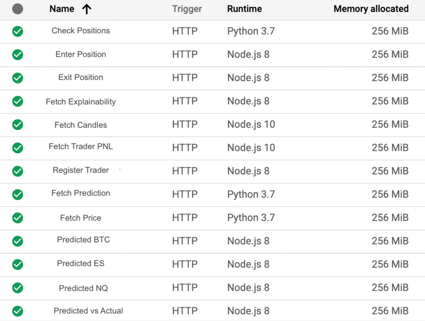
Figure 10 shows an inventory of the principal functions used in our market data pipelines.

Figure 10: Sample inventory of Cloud Functions

Many of these functions provide input to a machine learning model, while others fetch data from BigQuery for visualizations of trader performance in a real-time Profit/Loss ledger.

Conclusion

A data pipeline built from serverless components allows capital markets firms to focus on developing valuable insights and offerings, and not on managing infrastructure. In a serverless environment, the end users’ data access patterns can strongly influence the data pipeline architecture and schema design. This, in conjunction with a microservices architecture, minimizes code complexity and reduced coupling. As organizations continue to add data sources and information tools to their operations, using serverless computing models enable them to focus on value-added tasks of using data to make better decisions.

Learn more about Google Cloud for financial services.