Developers & Practitioners
Spring is here. Clocks move forward. The Sakura (cherry blossom) festival in Japan marks the celebration of the new season. In India, the holi festival of colors ushers in the new harvest season. It’s a time for renewal and new ways of doing things.
This month, we are pleased to debut our newest set of SQL features in BigQuery to help our analysts and data engineers spring forward. It’s time to set aside the old ways of doing things and instead look at these new ways of storing and analyzing all your data using BigQuery SQL.
Bigger data
Higher precision and more flexible functions to manage your ever-expanding data in BigQuery
BIGNUMERIC data type (GA)
We live in an era where intelligent devices and systems ranging from driverless vehicles to global stock and currency trading systems to high speed 5G networks are driving nearly all aspects of modern life. These systems rely on large amounts of precision data to perform real time analysis. To support these analytics, BigQuery is pleased to announce the general availability of BIGNUMERIC data type which supports 76 digits of precision and 38 digits of scale. Similar to NUMERIC, this new data type is available in all aspects of BigQuery from clustering to BI Engine and is also supported in the JDBC/ODBC drivers and client libraries.
Here is an example that demonstrates the additional precision and scale using BIGNUMERIC applied to the various powers of e, Euler’s number and the base of natural logarithms. Documentation
As an aside, did you know that the world record, as of December 5, 2020, for the maximum number of digits to represent e stands at 10? trillion digits?
SELECTx,EXP(CAST(x AS bignumeric)) exp_bignumeric,EXP(CAST(x AS float64)) exp_float,EXP(CAST(x as numeric)) exp_numericFROMUNNEST([1, 2, 10]) x;
JSON extraction functions (GA)
As customers analyze different types of data, both structured and semi-structured, within BigQuery, JavaScript Object Notation (JSON) has emerged as the de facto standard for semi-structured data. JSON provides the flexibility of storing schemaless data in tables without requiring the specification of data types with associated precision for columns. As new elements are added, the JSON document can be extended to add new key-value pairs without requiring schema changes.
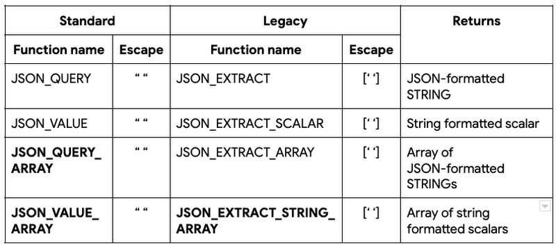
BigQuery has long supported JSON data and JSON functions to query and transform JSON data before they became a part of the ANSI SQL standard in 2016. JSON extraction functions typically take two parameters: JSON field, which contains the JSON document and JSONPath, which points to the specific element or array of elements that need to be extracted. If JSONPath references an element or elements containing reserved characters, such as dot(.), dollar($) or star(*) characters, they need to be escaped so that they can be treated as strings instead of being interpreted as JSONPath expressions. To support escaping, BigQuery supports two types of JSON extraction functions: Standard and Legacy. The Standard (ANSI compliant and recommended) way of escaping these reserved characters is by enclosing the reserved characters in double quotes (” “). The Legacy (pre-ANSI) way is to enclose them in square brackets and single quotes ([‘ ‘]).
Here’s a quick summary of existing and the new (highlighted in bold) JSON extraction functions:
WITH table AS(SELECT '{"list": ["book", "apple", "pen"]}' AS json_string UNION ALLSELECT '{"list": [{"name": "book"}, {"name:": "apple"}]}' AS json_string UNION ALLSELECT '{"list": [10, "apple", true]}' AS json_string)SELECT JSON_QUERY(json_string, "$.list[0]") AS json_query,JSON_VALUE(json_string, "$.list[0]") AS json_value,JSON_QUERY_ARRAY(json_string, "$.list") AS json_query_array,JSON_VALUE_ARRAY(json_string, "$.list") AS json_value_arrayFROM table;WITH table AS(SELECT '{"first.name": "Alice"}' AS json_string)SELECT JSON_EXTRACT_SCALAR(json_string, "$['first.name']") AS json_extract_scalar,JSON_VALUE(json_string, '$."first.name"') AS json_valueFROM table;
TABLESAMPLE clause (preview)
With the convergence into and growth of all types of data within BigQuery, customers want to maintain control over query costs especially when analysts and data scientists are performing ad hoc analysis of data in large tables. We are pleased to introduce the TABLESAMPLE clause in queries which allows users to sample a subset of the data, specified as a percentage of a table, instead of querying the entire data from large tables. This SQL clause can sample data from native BigQuery tables or external tables, stored in storage buckets in Google Cloud Storage, by randomly selecting a percentage of data blocks from the table and reading all of the rows in the selected blocks, lowering query costs when trying ad hoc queries. Documentation
SELECT *FROM `bigquery-public-data`.crypto_dogecoin.transactions tablesample system (10 percent)WHERE block_timestamp_month = '2019-01-01';
Agile schema
More commands and capabilities in SQL to allow you to evolve your data as your analytics needs change.
Dataset (SCHEMA) operations (GA)
In BigQuery, a dataset is the top level container entity that contains the data and program objects, such as tables, views, procedures. Creating, maintaining and dropping these datasets have been supported thus far in BigQuery using API, cli and UI. Today, we’re pleased to offer full SQL support (CREATE, ALTER and DROP) for dataset operations using SCHEMA, the ANSI standard keyword for the collection of logical objects in a database or a data warehouse. These operations greatly simplify data administrators’ ability to provision and manage schema across their BigQuery projects. Documentation for CREATE, ALTER and DROP SCHEMA syntax
# Replace myproject and mydataset with your preferred project and dataset names# Create a schema and set some optionsCREATE SCHEMA IF NOT EXISTS myproject.mydataset OPTIONS(default_table_expiration_days=22,default_partition_expiration_days=5.3,Friendly_NAME="DDL schema",DESCRIPTION="A schema for testing DDL options",labels=[("k1", "v1"), ("k2", "v2")]);# Create a table belonging to this schemaCREATE TABLE myproject.mydataset.my_table (x INT64, y STRING);# Alter the schema to change table expiration dateALTER SCHEMA IF EXISTS myproject.mydataset SET OPTIONS(default_table_expiration_days=7,DESCRIPTION="new description",labels=[("k1", "v1"), ("k2", "v2")]);# Dropping this dataset (schema) will give a warning message since it is not empty.DROP SCHEMA myproject.mydataset RESTRICT;# Drop this dataset (schema) and its contentsDROP SCHEMA myproject.mydataset CASCADE;
Object creation DDL from INFORMATION_SCHEMA (preview)
Data administrators provision empty copies of production datasets to allow loading of fictitious data so that developers can test out new capabilities before they are added to production datasets; new hires can train themselves on production-like datasets with test data. To help data administrators generate the data definition language (DDL) for objects, the TABLES view in INFORMATION_SCHEMA in BigQuery now has a new column called DDL which contains the exact object creation DDL for every table, view and materialized view within the dataset. In combination with dynamic SQL, data administrators can quickly generate and execute the creation DDL commands for a specific object or all objects of particular type, e.g. MATERIALIZED VIEW or all data objects within a specified dataset with a single SQL statement without having to manually reconstruct all options and elements associated with the schema object(s). Documentation
# Note that the object creation DDL captures the entire object definition,# including table structure, options, description and commentsSELECTtable_name, ddlFROM`bigquery-public-data`.census_bureau_usa.INFORMATION_SCHEMA.TABLES;
DROP COLUMN support (preview)
In October 2020, BigQuery introduced ADD COLUMN support in SQL to allow users to add columns using SQL to existing tables. As data engineers and analysts expand their tables to support new data, some columns may become obsolete and need to be removed from the tables. BigQuery now supports the DROP COLUMN clause as a part of the ALTER TABLE command to allow users to remove one or more of these columns. During the Preview period, note that there are certain restrictions on DROP COLUMN operations that will remain in effect. See Documentation for more details.
# Replace myproject and mydemo1 with your preferred project and dataset names# 1. Create a table with some data.CREATE OR REPLACE TABLE mydataset.dropColumnTableASSELECT * FROM `bigquery-public-data.covid19_open_data.covid19_open_data`LIMIT 1000;# 2. Drop existing columns and a non existing column.ALTER TABLE mydataset.dropColumnTableDROP COLUMN iso_3166_1_alpha_2,DROP COLUMN IF EXISTS iso_3166_1_alpha_3,DROP COLUMN IF EXISTS nonExistingCol;
Longer column names (GA)
BigQuery now allows you to have longer column names upto 300 characters within tables, views and materialized views instead of the previous limit of 128 characters. Documentation
# Replace myproject and mydemo1 with your preferred project and dataset names# 1. Create a table with a very long column name.CREATE OR REPLACE TABLE mydataset.tablenameASSELECT date, location_key, aggregation_levelFROM `bigquery-public-data.covid19_open_data.covid19_open_data`LIMIT 1000;#2. Add a very long column name ( > 128 chars & <= 300 chars) to keep notes with each row.ALTER TABLE mydataset.tablenameADD COLUMN this__extra__long__column__name__is__intended__for__additional__notes__collected__from__the__public__breifing__by__local__officials__and__county__officials__and__state__officials__and__country__officials__so__that__it__can__be__extended__to__its__full__extended__length__allowed__by__bigquery__period STRING;# 2. Insert data into the table.UPDATE mydataset.tablenameSET this__extra__long__column__name__is__intended__for__additional__notes__collected__from__the__public__breifing__by__local__officials__and__county__officials__and__state__officials__and__country__officials__so__that__it__can__be__extended__to__its__full__extended__length__allowed__by__bigquery__period = "No Notes"WHERE true;# 3. Query date and notes from the table.SELECT date, this__extra__long__column__name__is__intended__for__additional__notes__collected__from__the__public__breifing__by__local__officials__and__county__officials__and__state__officials__and__country__officials__so__that__it__can__be__extended__to__its__full__extended__length__allowed__by__bigquery__periodFROM mydataset.tablenameLIMIT 100;
Storage insights
Storage usage analysis for partitioned and unpartitioned tables
INFORMATION_SCHEMA.PARTITIONS view for tables (preview)
Customers store their analytical data in tables within BigQuery and use the flexible partitioning schemes on large tables in BigQuery to organize their data for improved query efficiency. To provide data engineers with better insight on storage and the record count for tables, partitioned and unpartitioned, we are pleased to introduce PARTITIONS view as a part of BigQuery INFORMATION_SCHEMA. This view provides up-to-date information on tables or partitions of a table, such as the size of the table (logical and billable bytes), number of rows, the last time the table (or partition) was updated and whether the specific table (or partition) or is active or has aged out into cheaper long term storage. Partition entries for tables are identified by their PARTITION_ID while unpartitioned tables have a single NULL entry for PARTITION_ID.
Querying INFORMATION_SCHEMA views is more cost-efficient compared to querying base tables. Thus, the PARTITIONS view can be used in conjunction with queries to filter the query to specific partitions, e.g. finding data in the most recently updated partition or the maximum value of a partition key, as shown in the example below. Documentation
-- This query scans 1.6 GB, the single partition plus 10MB for querying-- INFORMATION_SCHEMA. The table must be partitioned and clusteredSELECT count(*) FROM `bigquery-public-data.worldpop.population_grid_1km`WHERE last_updated = (SELECT MAX(PARSE_DATE("%Y%m%d", partition_id))FROM `bigquery-public-data.worldpop.INFORMATION_SCHEMA.PARTITIONS`WHERE table_name = "population_grid_1km");-- This query scans 34 GB since it reads the entire table.SELECT count(*) FROM `bigquery-public-data.worldpop`.population_grid_1kmWHERE last_updated = (SELECT MAX(last_updated)FROM `bigquery-public-data.worldpop`.population_grid_1km);
We hope these new capabilities put a spring in the step of our BigQuery users as we continue to work hard to bring you more user-friendly SQL. To learn more about BigQuery, visit our website, and get started immediately with the free BigQuery Sandbox.