MegaCortex | Malware Authors Serve Up Bad Tasting Ransomware
July 25, 2019The Good, the Bad and the Ugly in Cybersecurity – Week 30
July 26, 2019Data Analytics
WorkplaceTransformation-01.png
Editor’s note: Today’s post comes from Or Hiltch, co-founder and CTO at Skyline AI, an investment manager for commercial real estate. Or describes how BigQuery ML can be used to perform unsupervised anomaly detection.
Anomaly detection is the process of identifying data or observations that deviate from the common behavior and patterns of our data, and is used for a variety of purposes, such as detecting bank fraud or defects in manufacturing. There are many approaches to anomaly detection and choosing the right method has a lot to do with the type of data we have. Since detecting anomalies is a fairly generic task, a number of different machine learning algorithms have been created to tailor the process to specific use cases.
Here are a few common types:
- Detecting suspicious activity in a time series, for example a log file. Here, the dimension of time plays a huge role in the data analysis to determine what is considered a deviation from normal patterns.
- Detecting credit card fraud based on a feed of transactions in a labeled dataset of historical frauds. In this type of supervised learning problem, we can train a classifier to classify a transaction as anomalous or fraudulent given that we have a historical dataset of known transactions, authentic and fraudulent.
- Detecting a rare and unique combination of a real estate asset’s attributes — for instance, an apartment building from a certain vintage year and a rare unit mix. At Skyline AI, we use these kinds of anomalies to capture interesting rent growth correlations and track down interesting properties for investment.

When applying machine learning for anomaly detection, there are primarily three types of setups: supervised, semi-supervised and unsupervised. In our case, we did not have enough labeled data depicting known anomalies in advance, so we used unsupervised learning.
In this post, we’ll demonstrate how to implement a simple unsupervised anomaly detection algorithm using BigQuery, without having to write a single line of code outside of BigQuery’s SQL.
K-means clustering — Using unsupervised machine learning for anomaly detection
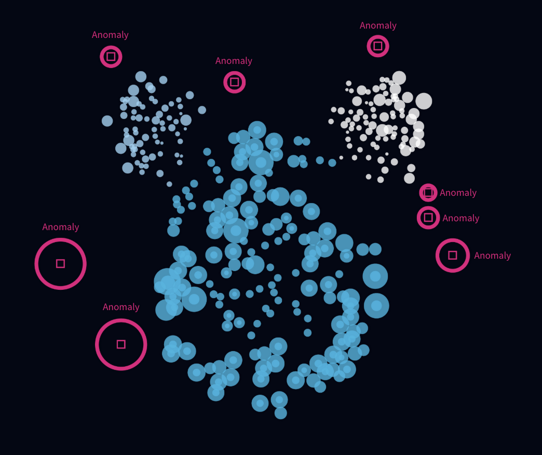
One method of finding anomalies is by generating clusters in our data and analyzing those clusters. A clustering algorithm is an algorithm that, given n points over a numeric space, will find the best way to split them into k groups. The definition of the best way may vary by the type of algorithm, but in this post we’ll focus on what it means for K-Means clustering.
If we organize the groups so that the “center of mass” in each group represents the “purest” characteristics of that group, the closer a data point is to that center would indicate whether it is more “standard” or “average” when compared to other points in the group . This allows us to analyze each group and ask ourselves, which points in the group are furthest away from the center of mass, and therefore, the most odd?
In general, when clustering, we seek to:
- Minimize the maximum radius of a cluster. If our data contains a lot of logical differences, we want to capture these with as many clusters as possible.
- Maximize the average inter-cluster distance. We want our clusters to be different from each other. If our clusters don’t represent differences well enough, they are useless.
- Minimize the variance within each cluster. Within each cluster, we want the data points to be as similar to each other as possible — this is what makes them members of the same group.
K-Means, an unsupervised learning algorithm, is one of the most popular clustering algorithms. If you’d like to learn more about the internals of how K-Means works, I would recommend walking through this great lab session.
The Iris Dataset
The Iris dataset is one of the “hello world” datasets for ML, consisting of 50 samples from each of three species of Iris (Iris setosa, Iris virginica and Iris versicolor). Four features were measured from each sample: the length and the width of the sepals and petals, in centimeters. Based on the combination of these four features, statistician and biologist Ronald Fisher developed a linear discriminant model to distinguish the species from each other.
In this tutorial, we’ll be detecting anomalies within the Iris dataset. We will find the rarest combinations of sepal and petal lengths and widths for the given species if Iris. The dataset can be obtained here.
Creating the clusters with BigQuery ML
BigQuery ML lets us create and execute machine learning models in BigQuery using standard SQL queries. It uses the output of SQL queries as input for a training process for machine learning algorithms, including k-means, and for generating predictions using those models, all within BigQuery.
After loading the Iris dataset into a table called public.iris_clusters, we can use the CREATE OR REPLACE MODEL statement to create a k-means model:
CREATE OR REPLACE MODELpublic.iris_clustersOPTIONS(model_type='kmeans',num_clusters=4,standardize_features = TRUE) ASSELECTDISTINCT sepal_length,sepal_width,petal_length,petal_width,speciesFROM`public.iris`
You can find more information on how to tune the model, and more, here.
Detecting anomalies in the clusters
Now that we have our clusters ready using BigQuery, how do we detect anomalies? Recall that in k-means, the closer a data point is to the center of the cluster (the “center of mass”), the more “average” it is compared to other data points in the cluster. This center is called centroid. One approach we could take to find anomalies in the data is to find those data points which are furthest away from the centroid of their cluster.
Getting the distances of each point from its centroid
The ML.PREDICT function of a k-means model in BigQuery returns an array containing each data point and its distance from the closest centroids. Using the UNNEST function we can flatten this array, taking only the minimum distance (the distance to the closest centroid):
WITHDistances AS (SELECTDISTINCT ML.CENTROID_ID,sepal_length,sepal_width,petal_length,petal_width,species,MIN(NEAREST_CENTROIDS_DISTANCE.DISTANCE) AS distance_from_closest_centroidFROMML.PREDICT(MODEL public.iris_clusters,(SELECTDISTINCT sepal_length,sepal_width,petal_length,petal_width,speciesFROM`public.iris` )) AS MLCROSS JOINUNNEST(NEAREST_CENTROIDS_DISTANCE) AS NEAREST_CENTROIDS_DISTANCEGROUP BYML.CENTROID_ID,sepal_length,sepal_width,petal_length,petal_width,species )
Setting a threshold for anomalies and grabbing the outliers
After we prepared the Distances table, we are ready to find the outliers — the data points farthest away from their centroid in each cluster.
To do this, we can use BigQuery’s Approximate Aggregate Functions to compute the 95th percentile. The 95th percentile tells you the value for which 95% of the data points are smaller and 5% are bigger. We will look for those 5% bigger ones:
Threshold AS (SELECTROUND(APPROX_QUANTILES(distance_from_closest_centroid,10000)[OFFSET(9500)],2) AS thresholdFROMDistances)
Putting It All Together
Using Distances and Threshold together, we finally detect the anomalies in one query:
WITHDistances AS (SELECTDISTINCT ML.CENTROID_ID,sepal_length,sepal_width,petal_length,petal_width,species,MIN(NEAREST_CENTROIDS_DISTANCE.DISTANCE) AS distance_from_closest_centroidFROMML.PREDICT(MODEL public.iris_clusters,(SELECTDISTINCT sepal_length,sepal_width,petal_length,petal_width,speciesFROM`public.iris` )) AS MLCROSS JOINUNNEST(NEAREST_CENTROIDS_DISTANCE) AS NEAREST_CENTROIDS_DISTANCEGROUP BYML.CENTROID_ID,sepal_length,sepal_width,petal_length,petal_width,species ),Threshold AS (SELECTROUND(APPROX_QUANTILES(distance_from_closest_centroid,10000)[OFFSET(9500)],2) AS thresholdFROMDistances)SELECTd.*FROMDistances dJOINThresholdONd.distance_from_closest_centroid > Threshold.threshold
The above query produces the following resultset:
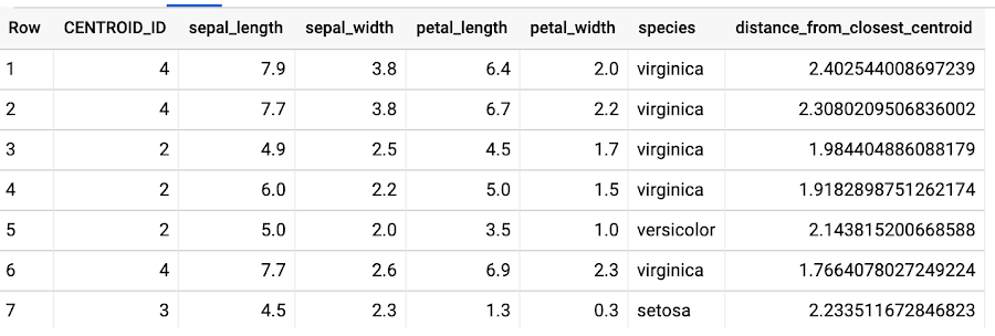
Let’s check how rare some of these anomalies really are. For the species of Iris virginica, how rare is a sepal length of 7.7, sepal width of 2.6, petal length of 6.9 and petal width of 2.3?
Let’s plot a histogram of the features for the species virginica. Note the green bars to represent the anomaly described above:
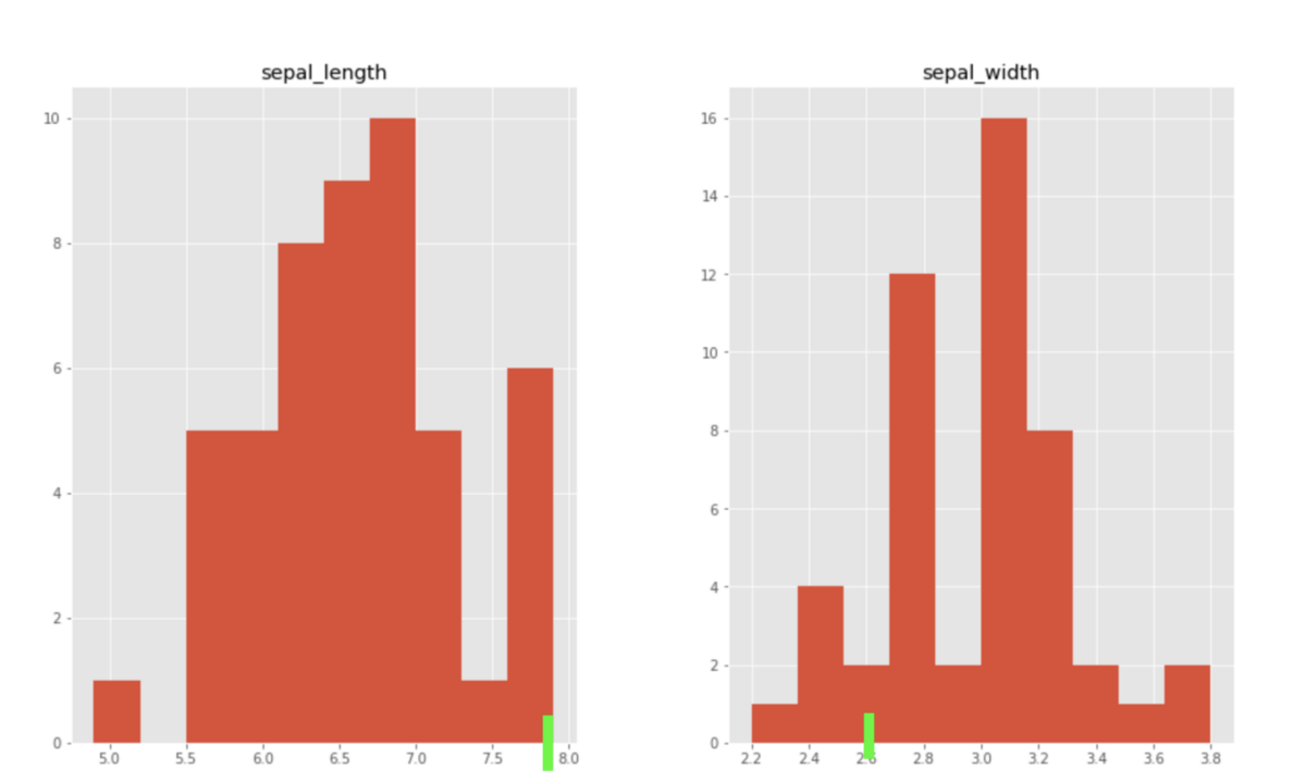
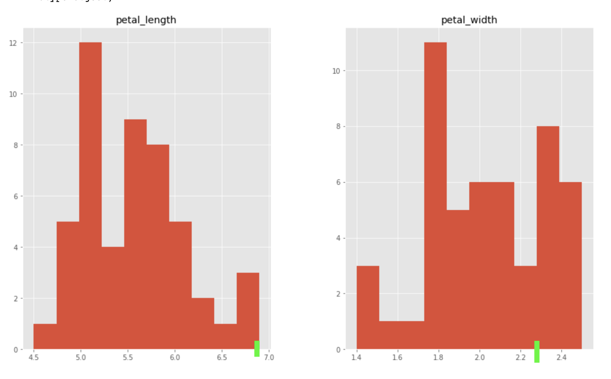
While it’s hard to mentally imagine the rarity of a combination of a 4-dimensional array, it can be seen in the histograms that this sample is indeed quite rare.
Summary

We’ve seen how several features of BigQuery — BigQuery ML, Approximate Aggregate Function and Arrays, can converge into one simple and powerful anomaly detection application, with a wide variety of use cases, and all without requiring us to write a single line of non-SQL code outside of BigQuery.
All of these features of BigQuery combined empower data analysts and engineers to use AI through existing SQL skills. You no longer need to export large amounts of data to spreadsheets or other applications, and in many cases, analysts no longer need to wait for limited resources from a data science team.
To learn more about k-means clustering on BigQuery ML, read the documentation.


