How to serve deep learning models using TensorFlow 2.0 with Cloud Functions

IBM Closes Landmark Acquisition of Red Hat for $34 Billion; Defines Open, Hybrid Cloud Future

July 9, 2019

Accelerating High Performance Computing (HPC) solutions in the cloud from Proof of Concept to Production

July 9, 2019

AI & Machine Learning

CloudFunctions_TF.png

Rustem Feyzkhanov

Machine Learning Engineer, Instrumental

July 9, 2019

Try GCP

Get $300 free credit to spend over 12 months.

Free Trial

Editor’s note: Today’s post comes from Rustem Feyzkhanov, a machine learning engineer at Instrumental. Rustem describes how Cloud Functions can be used as inference for deep learning models trained on TensorFlow 2.0, the advantages and disadvantages of using this approach, and how it is different from other ways of deploying the model.

TensorFlow is an established framework for training and inference of deep learning models. Recent updates to version 2.0 offer a number of enhancements, including significant changes to eager execution. But one of the challenges with this new framework is deploying TensorFlow 2.0 deep learning models. Google Cloud Functions offer a convenient, scalable and economic way of running inference within Google Cloud infrastructure and allows you to run the most recent version of this framework.

This post will explain how to run inference on Cloud Functions using TensorFlow 2.0.

We’ll explain how to deploy a deep learning inference including:

How to install and deploy Cloud Functions
How to store a model
How to use the Cloud Functions API endpoint

The components of our system

Google Cloud Platform (GCP) provides multiple ways for deploying inference in the cloud. Let’s compare the following methods for deploying the model:

Compute Engine cluster with TF serving
Cloud AI Platform Predictions
Cloud Functions

TensorFlow Serving
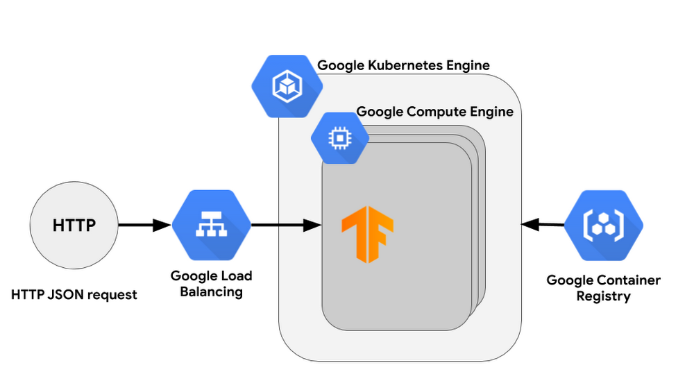
Typically you might use a cluster as inference for the model. In this case, TF serving would be a great way to organize inference on one or more VMs –then, all you need to do is add a load balancer on top of the cluster. You can use the following products to deploy TF serving in AI Platform:

This approach has the following advantages:

Great response time as the model will be loaded in the memory
Economy of scale, meaning cost per run will decrease significantly when you have a lot of requests

AI Platform Predictions
AI Platform provides an easy way to serve pre-trained models through AI Platform Predictions. This has many advantages for inference when compared to the cluster approach:

Codeless inference makes getting started easy
Scalable infrastructure
No management of infrastructure required
Separate storage for the model, which is very convenient for tracking versions of the model and for comparing their performance

Note: You can use Cloud Functions in combination with AI Platform Predictions (you can learn more in this post).

Cloud Functions
When comparing Deep Learning VMs and AI Platform Predictions, the full serverless approach provides the following advantages:

Simple code for implementing the inference, which at the same time allows you to implement custom logic.
Great scalability, which allows you to scale from 0 to 10k almost immediately
Cost structure which allows you only to pay for runs, meaning you don’t pay for idle servers.
Ability to use custom versions of different frameworks (Tensorflow 2.0 or PyTorch)

In summary, please take a look at this table:

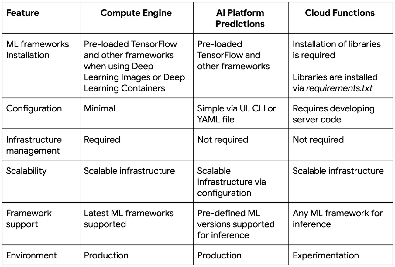
Since Google Cloud also provides some free invocations of Cloud Functions per month, this kind of setup would be perfect for a pet project or for a start-up that wants to get early customer feedback on a prototype. Also, it would be useful in cases where you have to process peak loads. The downside would be that in cases where the model is too big, the cold start could take some time and it would be very hard to achieve real-time performance. Also we need to keep in mind that serverless infrastructure doesn’t provide economy of scale, meaning the price of an individual run won’t go down when you have a large number of requests, so in these types of cases, it may be cheaper to use a cluster with TF serving as inference.

As we can see, Compute Engine pricing per hour looks extremely attractive (with utilizing preemptible instances or commitment use, the price will be even lower), but the catch here is that cost of instance is per one second, with a minimum of one minute. Cloud Functions, on the other hand, have billing per 100ms without a minimum time period. This means Cloud Functions are great for short, inconsistent jobs, but if you need to handle a long, consistent stream of jobs, Compute Engine might be a better choice.

Architecture Overview

Our system will be pretty simple. We will train the model locally and then upload it to Google Cloud. Cloud Functions will be invoked through an API request and will a download model and a test image from Cloud Storage.

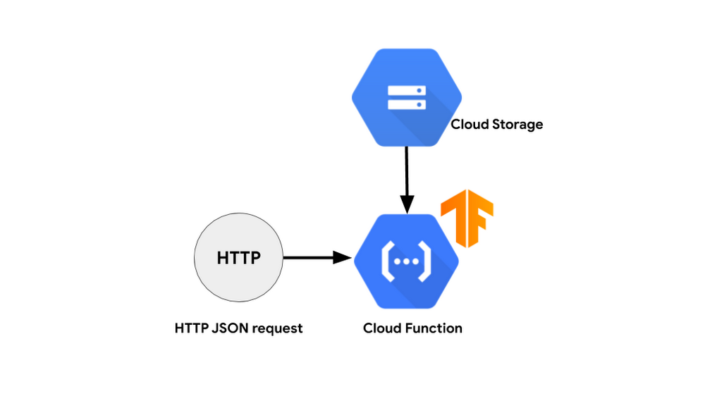
There are several things to consider when you design a system to use serverless infrastructure as an inference.

First of all, keep in mind differences between cold invocation, when the function needs time to download and initialize the model, and warm invocation, when function uses a cached model. Increasing the ratio of warm invocations to cold invocations not only allows you to increase processing speed, it also decreases the cost of your inference. There are multiple ways you can increase the ratio. One way could be warming up functions so they will be warm when a high load comes in. Another way is to use Pub/Sub to normalize a load so that it will be processed by warm containers.

Secondly, you can use batching to optimize the cost and speed of processing. Because a model can run on the whole batch instead of running separately on each image, batching allows you to decrease the difference between cold and warm invocation and improve overall speed.

Finally, you can have some part of your model saved as part of your libraries. This allows you to save time downloading the model during cold invocation. You could also try to divide the model into layers and chain them together on separate functions. In this case, each function will send an intermediate activation layer down the chain and neither of the functions would need to download the model.

Cost
In the demo which we will deploy we use 2GB Cloud Function. Cold invocation takes 3.5s and warn invocation takes 0.5s. In terms of pricing we get 0.0001019$ per cold invocation and 0.0000149$ per warm invocation. It means that for 1$ we get ~10k cold invocations and ~65k warm invocations. With free tier provided by Google Cloud you would get for free ~20k cold invocations and ~140k warm invocations per month. Feel free to check the pricing for your use cases using pricing calculator.

TensorFlow 2.0 example

First, let’s install Tensorflow 2.0 beta on your computer. You can install it either on your system python or by creating a virtual environment:

  pip install tensorflow==2.0.0b0

Let’s use fashion MNIST with TensorFlow 2.0b as an example. Here is how the code for training and exporting model weights would look like:

Based on the example:

  from __future__ import absolute_importfrom __future__ import divisionfrom __future__ import print_functionfrom __future__ import unicode_literalsimport tensorflow as tffrom tensorflow.keras.layers import Dense, Flatten, Conv2Dfrom tensorflow.keras import ModelEPOCHS = 10mnist = tf.keras.datasets.mnistfashion_mnist = tf.keras.datasets.fashion_mnist(x_train, y_train), (x_test, y_test) = fashion_mnist.load_data()x_train, x_test = x_train / 255.0, x_test / 255.0# Add a channels dimension e.g. (60000, 28, 28) => (60000, 28, 28, 1)x_train = x_train[..., tf.newaxis]x_test = x_test[..., tf.newaxis]train_ds = tf.data.Dataset.from_tensor_slices(    (x_train, y_train)).shuffle(10000).batch(32)test_ds = tf.data.Dataset.from_tensor_slices((x_test, y_test)).batch(32)class CustomModel(Model):  def __init__(self):    super(CustomModel, self).__init__()    self.conv1 = Conv2D(32, 3, activation='relu')    self.flatten = Flatten()    self.d1 = Dense(128, activation='relu')    self.d2 = Dense(10, activation='softmax')      def call(self, x):    x = self.conv1(x)    x = self.flatten(x)    x = self.d1(x)    return self.d2(x)model = CustomModel()loss_object = tf.keras.losses.SparseCategoricalCrossentropy()optimizer = tf.keras.optimizers.Adam()train_loss = tf.keras.metrics.Mean(name='train_loss')train_accuracy = tf.keras.metrics.SparseCategoricalAccuracy(name='train_accuracy')test_loss = tf.keras.metrics.Mean(name='test_loss')test_accuracy = tf.keras.metrics.SparseCategoricalAccuracy(name='test_accuracy')@tf.functiondef train_step(images, labels):  with tf.GradientTape() as tape:    predictions = model(images)    loss = loss_object(labels, predictions)  gradients = tape.gradient(loss, model.trainable_variables)  optimizer.apply_gradients(zip(gradients, model.trainable_variables))  train_loss(loss)  train_accuracy(labels, predictions)@tf.functiondef test_step(images, labels):  predictions = model(images)  t_loss = loss_object(labels, predictions)  test_loss(t_loss)  test_accuracy(labels, predictions)for epoch in range(EPOCHS):  for images, labels in train_ds:    train_step(images, labels)  for test_images, test_labels in test_ds:    test_step(test_images, test_labels)  template = 'Epoch {}, Loss: {}, Accuracy: {}, Test Loss: {}, Test Accuracy: {}'  print (template.format(epoch+1,                         train_loss.result(),                         train_accuracy.result()*100,                         test_loss.result(),                         test_accuracy.result()*100))# Save the weightsmodel.save_weights('fashion_mnist_weights')

The code will produce the following files:

  fashion_mnist_weights_new.indexfashion_mnist_weights.data-00000-of-00001

We will need to store the model separately from the code as there is a limit on local file size on the Cloud Functions. You can upload them to the Cloud Storage bucket along with the test image.

Cloud Functions

One of the main upsides of Cloud Functions is that you don’t have to manually generate the package. You can just use a requirements.txt file and list all used libraries there. Also, remember to have the model as a global variable in your python code so it will be cached and reused in warm invocations of Cloud Functions.

Therefore we will have two files:

requirements.txt

  # Function dependencies, for example:# package>=versiontensorflow==2.0.0b0google-cloud-storage==1.16.1Pillow==6.0.0

and main.py

  import numpyimport tensorflowfrom google.cloud import storagefrom tensorflow.keras.layers import Dense, Flatten, Conv2Dfrom tensorflow.keras import Modelfrom PIL import Image# We keep model as global variable so we don't have to reload it in case of warm invocationsmodel = Noneclass CustomModel(Model):  def __init__(self):    super(CustomModel, self).__init__()    self.conv1 = Conv2D(32, 3, activation='relu')    self.flatten = Flatten()    self.d1 = Dense(128, activation='relu')    self.d2 = Dense(10, activation='softmax')  def call(self, x):    x = self.conv1(x)    x = self.flatten(x)    x = self.d1(x)    return self.d2(x)def download_blob(bucket_name, source_blob_name, destination_file_name):    """Downloads a blob from the bucket."""    storage_client = storage.Client()    bucket = storage_client.get_bucket(bucket_name)    blob = bucket.blob(source_blob_name)    blob.download_to_filename(destination_file_name)    print('Blob {} downloaded to {}.'.format(        source_blob_name,        destination_file_name))def handler(request):    global model    class_names = ['T-shirt/top', 'Trouser', 'Pullover', 'Dress', 'Coat',               'Sandal', 'Shirt', 'Sneaker', 'Bag', 'Ankle boot']    # Model load which only happens during cold starts    if model is None:        download_blob('<your_bucket_name>', 'tensorflow/fashion_mnist_weights.index', '/tmp/fashion_mnist_weights.index')        download_blob('<your_bucket_name>', 'tensorflow/fashion_mnist_weights.data-00000-of-00001', '/tmp/fashion_mnist_weights.data-00000-of-00001')        model = CustomModel()        model.load_weights('/tmp/fashion_mnist_weights')        download_blob('<your_bucket_name>', 'tensorflow/test.png', '/tmp/test.png')    image = numpy.array(Image.open('/tmp/test.png'))    input_np = (numpy.array(Image.open('/tmp/test.png'))/255)[numpy.newaxis,:,:,numpy.newaxis]    predictions = model.call(input_np)    print(predictions)    print("Image is "+class_names[numpy.argmax(predictions)])        return class_names[numpy.argmax(predictions)]

Deployment through the command line

You can easily deploy and run Cloud Functions using gcloud.

  git clone https://github.com/ryfeus/gcf-packscd gcf-packs/tensorflow2.0/example/gcloud functions deploy handler --runtime python37 --trigger-http --memory 2048gcloud functions call handler

The response would be:

  executionId: omx2o2y27sm9result: Trouser

Deployment through the web console

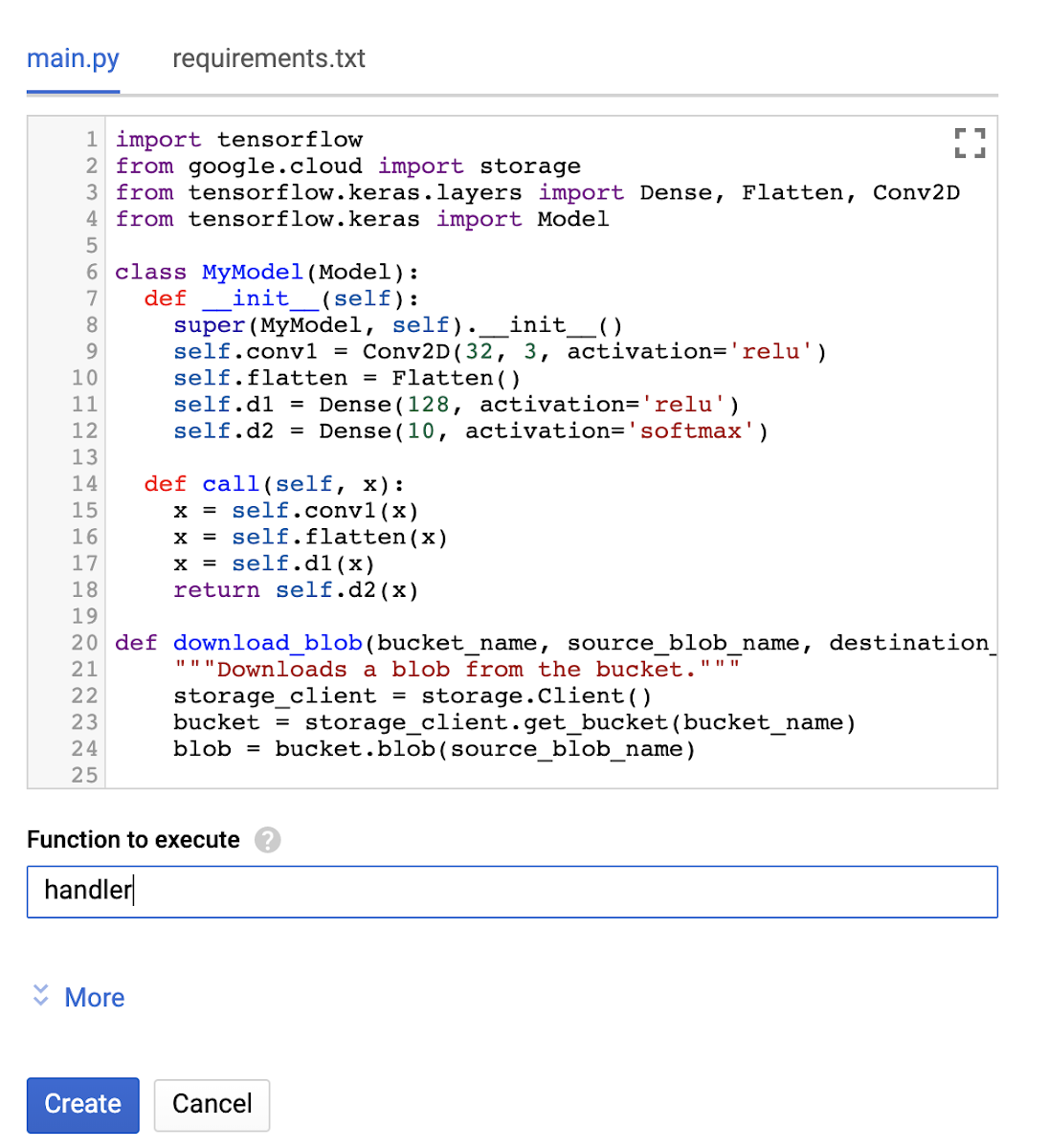
First, let’s start from the Cloud Functions dashboard. To create a new Cloud Function, choose the “Create function” button. In the “Create function” window, set the function’s name (“tensorflow2demo”), allocated memory (2 GB in our case for the best performance), trigger (HTTP trigger in our case) and runtime (python 3.7).

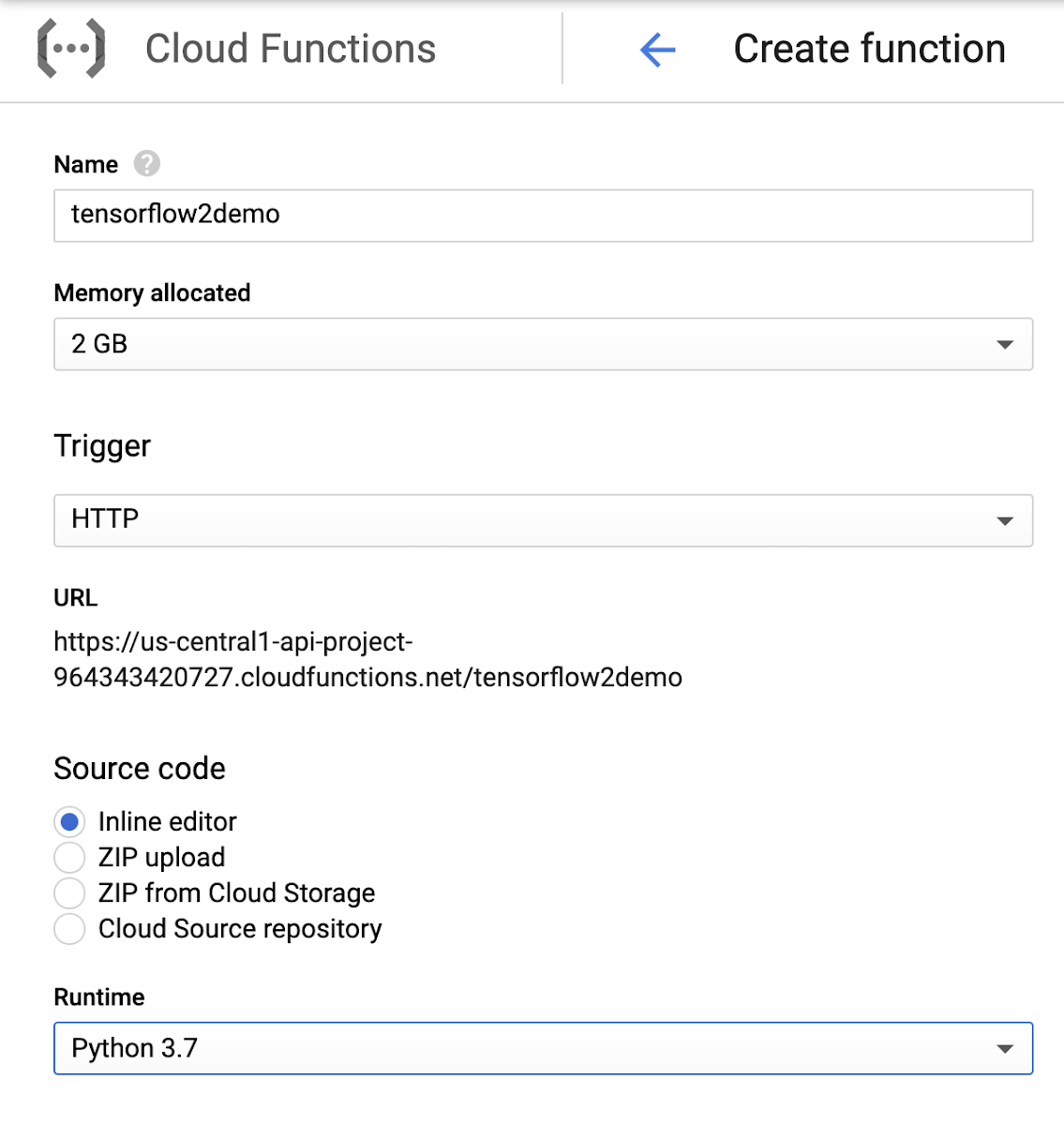
Next, set the main.py and requirements.txt files. You can just copy the code and libraries from the files at the repo. Finally, w push the “Create” button and initialize the creation of the function.

Once the function is deployed, you can test it in the “Testing” section of theCloud Functions dashboard. You can also customize incoming events and see output as well as logs.

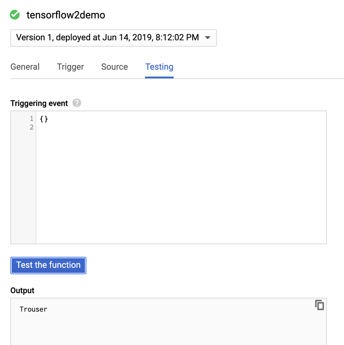
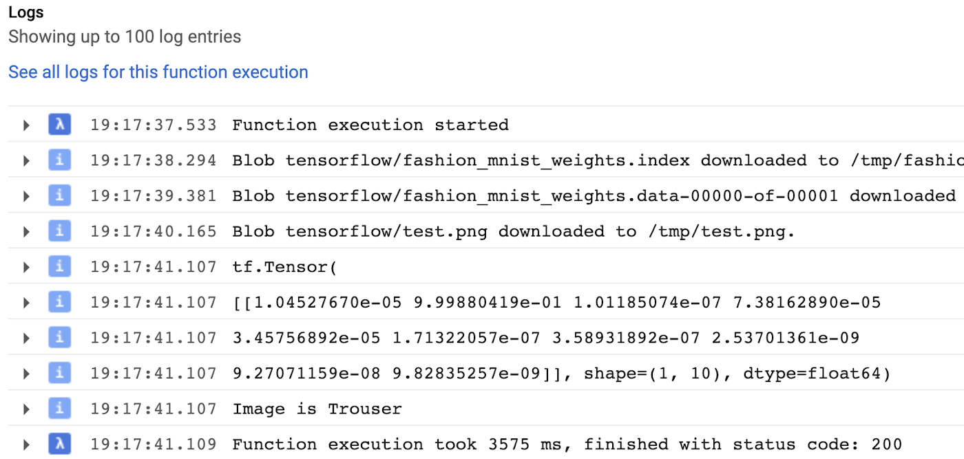
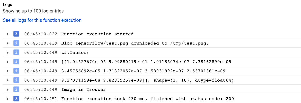
As you can see, our pretrained model successfully classified image as trousers. If we run the functions one more time, we will see that it will run a lot faster because we saved the model to the cache and won’t need to reload it during warm invocation.

Conclusion

With this post, you should now be able to create a TensorFlow 2.0 endpoint on GCloud Functions. Setting the project up is easy, and can save a lot of time when compared to the traditional approach of using a cluster of VMs. As you can see, Cloud Functions provide an easy way to start with contemporary frameworks and deploy pre-trained models in a matter of minutes.

As a hobby, I port a lot of libraries to make the serverless friendly. Feel free to check my repos with other examples like headless chrome or pandas with numpy on Cloud Functions. They all have an MIT license, so feel free to modify and use them for your project.

Learn more about Cloud Functions here, and consider starting a free trial.

Acknowledgements: Gonzalo Gasca Meza, Developer Programs Engineer contributed to this post.

Posted in: