AI & Machine Learning
nvidia.png
If you’re a data scientist, researcher, engineer, or developer, you may be familiar with Google Cloud’s set of Deep Learning Virtual Machine (VM) images, which enable the one-click setup machine learning-focused development environments. But some data scientists still use a combination of pandas, Dask, scikit-learn, and Spark on traditional CPU-based instances. If you’d like to speed up your end-to-end pipeline through scale, Google Cloud’s Deep Learning VMs now include an experimental image with RAPIDS, NVIDIA’s open source and Python-based GPU-accelerated data processing and machine learning libraries that are a key part of NVIDIA’s larger collection of CUDA-X AI accelerated software. CUDA-X AI is the collection of NVIDIA’s GPU acceleration libraries to accelerate deep learning, machine learning, and data analysis.
The Deep Learning VM Images comprise a set of Debian 9-based Compute Engine virtual machine disk images optimized for data science and machine learning tasks. All images include common machine learning (typically deep learning, specifically) frameworks and tools installed from first boot, and can be used out of the box on instances with GPUs to accelerate your data processing tasks. In this blog post you’ll learn to use a Deep Learning VM which includes GPU-accelerated RAPIDS libraries.
RAPIDS is an open-source suite of data processing and machine learning libraries developed by NVIDIA that enables GPU-acceleration for data science workflows. RAPIDS relies on NVIDIA’s CUDA language allowing users to leverage GPU processing and high-bandwidth GPU memory through user-friendly Python interfaces. It includes the DataFrame API based on Apache Arrow data structures called cuDF, which will be familiar to users of pandas. It also includes cuML, a growing library of GPU-accelerated ML algorithms that will be familiar to users of scikit-learn. Together, these libraries provide an accelerated solution for ML practitioners to use requiring only minimal code changes and no new tools to learn.
RAPIDS is available as a conda or pip package, in a Docker image, and as source code.
Using the RAPIDS Google Cloud Deep Learning VM image automatically initializes a Compute Engine instance with all the pre-installed packages required to run RAPIDS. No extra steps required!

Creating a new RAPIDS virtual machine instance
Compute Engine offers predefined machine types that you can use when you create an instance. Each predefined machine type includes a preset number of vCPUs and amount of memory, and bills you at a fixed rate, as described on the pricing page.
If predefined machine types do not meet your needs, you can create an instance with a custom virtualized hardware configuration. Specifically, you can create an instance with a custom number of vCPUs and amount of memory, effectively using a custom machine type.
In this case, we’ll create a custom Deep Learning VM image with 48 vCPUs, extended memory of 384 GB, 4 NVIDIA Tesla T4 GPUs and RAPIDS support.
export IMAGE_FAMILY="rapids-latest-gpu-experimental"export ZONE="us-central1-b"export INSTANCE_NAME="rapids-instance"export INSTANCE_TYPE="custom-48-393216-ext"gcloud compute instances create $INSTANCE_NAME--zone=$ZONE--image-family=$IMAGE_FAMILY--image-project=deeplearning-platform-release--maintenance-policy=TERMINATE--accelerator='type=nvidia-tesla-t4,count=4'--machine-type=$INSTANCE_TYPE--boot-disk-size=1TB--scopes=https://www.googleapis.com/auth/cloud-platform--metadata='install-nvidia-driver=True,proxy-mode=project_editors'
Notes:
- You can create this instance in any available zone that supports T4 GPUs.
- The option
install-nvidia-driver=TrueInstalls NVIDIA GPU driver automatically. - The option
proxy-mode=project_editorsmakes the VM visible in the Notebook Instances section. - To define extended memory, use 1024*X where X is the number of GB required for RAM.
Using RAPIDS
To put the RAPIDS through its paces on Google Cloud Platform (GCP), we focused on a common HPC workload: a parallel sum reduction test. This test can operate on very large problems (the default size is 2TB) using distributed memory and parallel task processing.
There are several applications that require the computation of parallel sum reductions in high performance computing (HPC). Some examples include:
- Solving linear recurrences
- Evaluation of polynomials
- Random number generation
- Sequence alignment
- N-body simulation
It turns out that parallel sum reduction is useful for the data science community at large. To manage the deluge of big data, a parallel programming model called “MapReduce” is used for processing data using distributed clusters. The “Map” portion of this model supports sorting: for example, sorting products into queues. Once the model maps the data, it then summarizes the output with the “Reduce” algorithm–for example, count the number of products in each queue. A summation operation is the most compute-heavy step, and given the scale of data that the model is processing, these sum operations must be carried out using parallel distributed clusters in order to complete in a reasonable amount of time.
But certain reduction sum operations contain dependencies that inhibit parallelization. To illustrate such a dependency, suppose we want to add a series of numbers as shown in Figure 1.

From the figure 1 on the left, we must first add 7 + 6 to obtain 13, before we can add 13 + 14 to obtain 27 and so on in a sequential fashion. These dependencies inhibit parallelization. However, since addition is associative, the summation can be expressed as a tree (figure 2 on the right). The benefit of this tree representation is that the dependency chain is shallow, and since the root node summarizes its leaves, this calculation can be split into independent tasks.
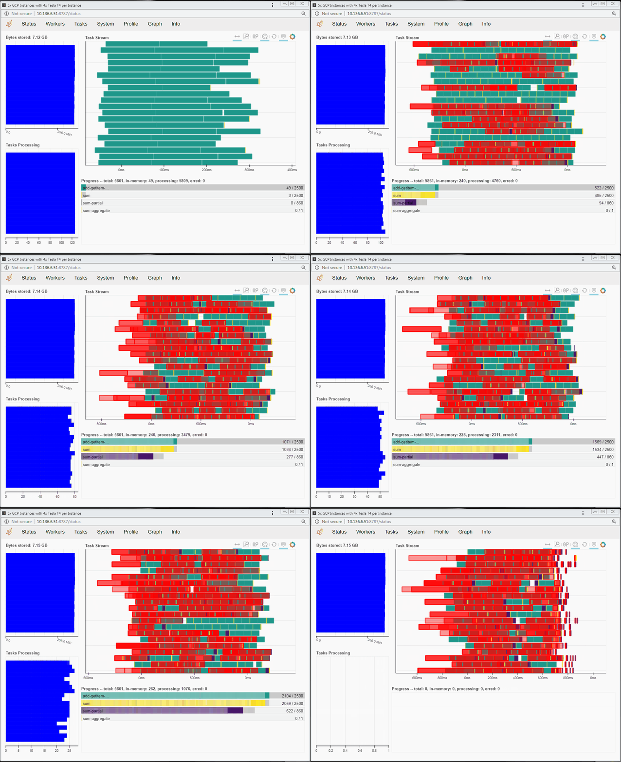
Speaking of tasks, this brings us to the Python package Dask, a popular distributed computing framework. With Dask, data scientists and researchers can use Python to express their problems as tasks. Dask then distributes these tasks across processing elements within a single system, or across a cluster of systems. The RAPIDS team recently integrated GPU support into a package called dask-cuda. When you import both dask-cuda and another package called CuPY, which allows data to be allocated on GPUs using familiar numpy constructs, you can really explore the full breadths of models you can build with your data set. To illustrate, shown in Figures 3 and 4 show side-by-side comparisons of the same test run. On the left, 48 cores of a single system are used to process 2 terabytes (TB) of randomly initialized data using 48 Dask workers. On the right, 4 Dask workers process the same 2 TB of data, but dask-cuda is used to automatically associate those workers with 4 Tesla T4 GPUs installed in the same system.
Running RAPIDS
To test parallel sum-reduction, perform the following steps:
1. SSH into the instance. See Connecting to Instances for more details.
2. Download the code required from this repository and upload it to your Deep Learning Virtual Machine Compute Engine instance. These two files are of particular importance as you profile performance:
You can find the sample code to run these tests, based on this blog, GPU Dask Arrays, below.
3. Run the tests:
Run test on the instance’s CPU complex, in this case specifying 48 vCPUs (indicated by the -c flag):
time ./run.sh -c 48Using CPUs and Local DaskAllocating and initializing arrays using CPU memoryArray size: 2.00 TB. Computing parallel sum . . .Processing complete.Wall time create data + computation time: 695.50063515 secondsreal 11m 45.523suser 0m 52.720ssys 0m 10.100s
Now, run the test using 4 (indicated by the -g flag) NVIDIA Tesla T4 GPUs:
time ./run.sh -g 4Using GPUs and Local DaskAllocating and initializing arrays using GPU memory with CuPYArray size: 2.00 TB. Computing parallel sum . . .Processing complete.Wall time create data + computation time: 57.94356680 secondsreal 1m 13.680suser 0m 9.856ssys 0m 13.832s


Here are some initial conclusions we derived from these tests:
- Processing 2 TB of data on GPUs is much faster (an ~12x speed-up for this test)
- Using Dask’s dashboard, you can visualize the performance of the reduction sum as it is executing
- CPU cores are fully occupied during processing on CPUs, but the GPUs are not fully utilized
- You can also run this test in a distributed environment
import argparseimport subprocessimport sysimport timeimport cupyimport dask.array as dafrom dask.distributed import Client, LocalCluster, waitfrom dask_cuda import LocalCUDAClusterdef create_data(rs, xdim, ydim, x_chunk_size, y_chunk_size):x = rs.normal(10, 1, size=(xdim, ydim),chunks=(x_chunk_size, y_chunk_size))return xdef run(data):(data + 1)[::2, ::2].sum().compute()returndef get_scheduler_info():scheduler_ip = subprocess.check_output(['hostname','--all-ip-addresses'])scheduler_ip = scheduler_ip.decode('UTF-8').split()[0]scheduler_port = '8786'scheduler_uri = '{}:{}'.format(scheduler_ip, scheduler_port)return scheduler_ip, scheduler_uridef main():parser = argparse.ArgumentParser()parser.add_argument('--xdim', type=int, default=500000)parser.add_argument('--ydim', type=int, default=500000)parser.add_argument('--x_chunk_size', type=int, default=10000)parser.add_argument('--y_chunk_size', type=int, default=10000)parser.add_argument('--use_gpus_only', action="store_true")parser.add_argument('--n_gpus', type=int, default=1)parser.add_argument('--use_cpus_only', action="store_true")parser.add_argument('--n_sockets', type=int, default=1)parser.add_argument('--n_cores_per_socket', type=int, default=1)parser.add_argument('--use_dist_dask', action="store_true")args = parser.parse_args()sched_ip, sched_uri = get_scheduler_info()if args.use_dist_dask:print('Using Distributed Dask')client = Client(sched_uri)elif args.use_gpus_only:print('Using GPUs and Local Dask')cluster = LocalCUDACluster(ip=sched_ip,n_workers=args.n_gpus)client = Client(cluster)elif args.use_cpus_only:print('Using CPUs and Local Dask')cluster = LocalCluster(ip=sched_ip,n_workers=args.n_sockets,threads_per_worker=args.n_cores_per_socket)client = Client(cluster)start = time.time()if args.use_gpus_only:print('Allocating arrays using GPU memory with CuPY')rs=da.random.RandomState(RandomState=cupy.random.RandomState)elif args.use_cpus_only:print('Allocating arrays using CPU memory')rs = da.random.RandomState()x = create_data(rs, args.xdim, args.ydim,args.x_chunk_size, args.y_chunk_size)print('Array size: {:.2f}TB. Computing...'.format(x.nbytes/1e12))run(x)end = time.time()delta = (end - start)print('Processing complete.')print('Wall time: {:10.8f} seconds'.format(delta))del xif __name__ == '__main__':main()
In this example, we allocate Python arrays using the double data type by default. Since this code allocates an array size of (500K x 500K) elements, this represents 2 TB (500K x 500K x 8 bytes / word). Dask initializes these array elements randomly via normal Gaussian distribution using the dask.array package.
Running RAPIDS on a distributed cluster
You can also run RAPIDS in a distributed environment using multiple Compute Engine instances. You can use the same code to run RAPIDS in a distributed way with minimal modification and still decrease the processing time. If you want to explore RAPIDS in a distributed environment please follow the complete guide here.
time ./run.sh -g 20 -dUsing Distributed DaskAllocating and initializing arrays using GPU memory with CuPYArray size: 2.00 TB. Computing parallel sum . . .Processing complete.Wall time create data + computation time: 11.63004732 secondsreal 0m 12.465suser 0m 1.432ssys 0m 0.324s


Conclusion
As you can see from the above example, the RAPIDS VM Image can dramatically speed up your ML workflows. Running RAPIDS with Dask lets you seamlessly integrate your data science environment with Python and its myriad libraries and wheels, HPC schedulers such as SLURM, PBS, SGE, and LSF, and open-source infrastructure orchestration projects such as Kubernetes and YARN. Dask also helps you develop your model once, and adaptably run it on either a single system, or scale it out across a cluster. You can then dynamically adjust your resource usage based on computational demands. Lastly, Dask helps you ensure that you’re maximizing uptime, through fault tolerance capabilities intrinsic in failover-capable cluster computing.
It’s also easy to deploy on Google’s Compute Engine distributed environment. If you’re eager to learn more, check out the RAPIDS project and open-source community website, or review the RAPIDS VM Image documentation.
Acknowledgements: Ty McKercher, NVIDIA, Principal Solution Architect; Vartika Singh, NVIDIA, Solution Architect; Gonzalo Gasca Meza, Google, Developer Programs Engineer; Viacheslav Kovalevskyi, Google, Software Engineer


